data

link

Column name	Original column name	Details
sample_id	Sample ID	Unique string identifying each subject
patient_cohort	Patient’s Cohort	Cohort 1: previously used samples; Cohort 2: newly added samples
sample_origin	Sample Origin	BPTB: Barts Pancreas Tissue Bank, London, UK; ESP: Spanish National Cancer Research Centre, Madrid, Spain; LIV: Liverpool University, UK; UCL: University College London, UK
age	Age	Age in years
sex	Sex	M = male, F = female
diagnosis	Diagnosis (1=Control, 2=Benign, 3=PDAC)	1 = control (no pancreatic disease), 2 = benign hepatobiliary disease (119 of which are chronic pancreatitis), 3 = Pancreatic ductal adenocarcinoma (pancreatic cancer)
stage	Stage	For those with pancreatic cancer, one of IA, IB, IIA, IIIB, III, IV
benign_sample_diagnosis	Benign Samples Diagnosis	For those with a benign, non-cancerous diagnosis, what was the diagnosis?
plasma_CA19_9	Plasma CA19-9 U/ml	Blood plasma levels of CA 19–9, often elevated in pancreatic cancer. Only assessed in 350 patients.
creatinine	Creatinine mg/ml	Urinary biomarker of kidney function
LYVE1	LYVE1 ng/ml	Urinary levels of Lymphatic vessel endothelial hyaluronan receptor 1, may play a role in tumor metastasis
REG1B	REG1B ng/ml	Urinary levels of a protein that may be associated with pancreas regeneration
TFF1	TFF1 ng/ml	Urinary levels of Trefoil Factor 1, related to regeneration and repair of urinary tract
REG1A	REG1A ng/ml	Urinary levels of a protein associated with pancreas regeneration. Only assessed in 306 patients.

import pandas as pd
import numpy as np
import seaborn as sns
import matplotlib.pyplot as plt
# 통계 검정
from scipy.stats import f_oneway
from scipy.stats import chi2_contingency
# ml
from sklearn.model_selection import train_test_split
from sklearn.ensemble import RandomForestClassifier
from sklearn.metrics import classification_report, confusion_matrix, roc_auc_score
from sklearn.preprocessing import StandardScaler, LabelEncoder
from sklearn.pipeline import Pipeline
from sklearn.impute import SimpleImputer
# 모델 후보
from sklearn.linear_model import LogisticRegression
from sklearn.svm import SVC
# pytorch
import torch
import torch.nn as nn
import torch.optim as optim
from torch.utils.data import Dataset, DataLoader, random_split

from sklearn.preprocessing import StandardScaler
from sklearn.metrics import classification_report, confusion_matrix, ConfusionMatrixDisplay

Data

df = pd.read_csv('../../../delete/Debernardi et al 2020 data.csv')

df

	sample_id	patient_cohort	sample_origin	age	sex	diagnosis	stage	benign_sample_diagnosis	plasma_CA19_9	creatinine	LYVE1	REG1B	TFF1	REG1A
0	S1	Cohort1	BPTB	33	F	1	NaN	NaN	11.7	1.83222	0.893219	52.948840	654.282174	1262.000
1	S10	Cohort1	BPTB	81	F	1	NaN	NaN	NaN	0.97266	2.037585	94.467030	209.488250	228.407
2	S100	Cohort2	BPTB	51	M	1	NaN	NaN	7.0	0.78039	0.145589	102.366000	461.141000	NaN
3	S101	Cohort2	BPTB	61	M	1	NaN	NaN	8.0	0.70122	0.002805	60.579000	142.950000	NaN
4	S102	Cohort2	BPTB	62	M	1	NaN	NaN	9.0	0.21489	0.000860	65.540000	41.088000	NaN
...	...	...	...	...	...	...	...	...	...	...	...	...	...	...
585	S549	Cohort2	BPTB	68	M	3	IV	NaN	NaN	0.52026	7.058209	156.241000	525.178000	NaN
586	S558	Cohort2	BPTB	71	F	3	IV	NaN	NaN	0.85956	8.341207	16.915000	245.947000	NaN
587	S560	Cohort2	BPTB	63	M	3	IV	NaN	NaN	1.36851	7.674707	289.701000	537.286000	NaN
588	S583	Cohort2	BPTB	75	F	3	IV	NaN	NaN	1.33458	8.206777	205.930000	722.523000	NaN
589	S590	Cohort1	BPTB	74	M	3	IV	NaN	1488.0	1.50423	8.200958	411.938275	2021.321078	13200.000

590 rows × 14 columns

df.describe()

	age	diagnosis	plasma_CA19_9	creatinine	LYVE1	REG1B	TFF1	REG1A
count	590.000000	590.000000	350.000000	590.000000	590.000000	590.000000	590.000000	306.000000
mean	59.079661	2.027119	654.002944	0.855383	3.063530	111.774090	597.868722	735.281222
std	13.109520	0.804873	2430.317642	0.639028	3.438796	196.267110	1010.477245	1477.247724
min	26.000000	1.000000	0.000000	0.056550	0.000129	0.001104	0.005293	0.000000
25%	50.000000	1.000000	8.000000	0.373230	0.167179	10.757216	43.961000	80.692000
50%	60.000000	2.000000	26.500000	0.723840	1.649862	34.303353	259.873974	208.538500
75%	69.000000	3.000000	294.000000	1.139482	5.205037	122.741013	742.736000	649.000000
max	89.000000	3.000000	31000.000000	4.116840	23.890323	1403.897600	13344.300000	13200.000000

for col in df.select_dtypes(include=['object', 'category']).columns:
    print(f"\n📊 {col}")
    print(df[col].value_counts(dropna=False))


📊 sample_id
S1      1
S588    1
S302    1
S288    1
S497    1
       ..
S282    1
S321    1
S323    1
S363    1
S590    1
Name: sample_id, Length: 590, dtype: int64

📊 patient_cohort
Cohort1    332
Cohort2    258
Name: patient_cohort, dtype: int64

📊 sample_origin
BPTB    409
LIV     132
ESP      29
UCL      20
Name: sample_origin, dtype: int64

📊 sex
F    299
M    291
Name: sex, dtype: int64

📊 stage
NaN    391
III     76
IIB     68
IV      21
IB      12
IIA     11
II       7
IA       3
I        1
Name: stage, dtype: int64

📊 benign_sample_diagnosis
NaN                                                             382
Pancreatitis                                                     41
Pancreatitis (Chronic)                                           35
Gallstones                                                       21
Pancreatitis (Alcohol-Chronic)                                   11
Cholecystitis                                                     9
Serous cystadenoma - NOS                                          7
Abdominal Pain                                                    6
Choledocholiathiasis                                              6
Pancreatitis (Alcohol-Chronic-Pseuodcyst)                         4
Pancreatitis (Gallstone)                                          4
Pancreatitis (Pseudocyst)                                         4
Pancreatitis (Idiopathic)                                         4
Pancreatitis (Autoimmune)                                         3
Serous microcystic adenoma                                        3
Gallstones - Incidental                                           3
Cholecystitis (Chronic)                                           3
Premalignant lesions-Mucinous cystadenoma-NOS                     3
Gallstones                                                        2
Gallbladder polyps                                                2
Premalignant lesions-Adenoma-NOS                                  2
Pancreatitis (Chronic-Pseudocyst)                                 2
Cholecystitis (Chronic) Cholelithiasis                            2
Premalignant lesions-Villous adenoma-NOS                          2
Pancreatitis (Gallstone-Pseudocyst)                               1
Pancreatitis (Gallstone-Alcohol-Pseudocyst)                       1
Pancreato-jejunostomy Anastomoses Stricture                       1
Premalignant lesions-Tubulovillous adenoma-NOS                    1
Pancreatitis (Chronic) Choledocholithiasis                        1
Premalignant lesions-Mucinous cystadenocarcinoma-noninvasive      1
Pancreatitis (Hereditary-Chronic)                                 1
Pancreatitis (Hypertriglyceridemia)                               1
Pancreatitis (Idiopathic)                                         1
Premalignant lesions-Tubular adenoma-NOS                          1
Pancreatitis (Abscess)                                            1
Pancreatitis (Chronic) (Later became PDAC)                        1
Pancreatitis (Alcohol)                                            1
Biliary Stricture (Secondary to Stent)                            1
Cholecystitis                                                     1
Cholecystitis (Chronic) Cholesterolsis                            1
Choledochal Cyst                                                  1
Choledocholiathiasis                                              1
Cholelithiasis with adenomyomatous hyperplasia                    1
Duodenal Stricture                                                1
Duodenitis                                                        1
Gallbladder Porcelain                                             1
Gastritis                                                         1
Gastritis and Reflux                                              1
Ill defined lesion in uncinate process                            1
Ischaemic Common Bile Duct Stricture                              1
Pancreatitis                                                      1
Pancreatitis (Acute)                                              1
Simple benign liver cyst                                          1
Name: benign_sample_diagnosis, dtype: int64

crosstab between sex

ct = pd.crosstab(df['sex'], df['diagnosis_label'])
print(ct)

diagnosis_label  Benign  Control  PDAC
sex                                   
F                   101      115    83
M                   107       68   116

Within-sex Proportions

print("\nWithin-sex proportions (%):")
print((ct.div(ct.sum(axis=1), axis=0) * 100).round(2))


Within-sex proportions (%):
diagnosis_label  Benign  Control   PDAC
sex                                    
F                 33.78    38.46  27.76
M                 36.77    23.37  39.86

남성이 많이 췌장암 발생하는 경향
성별 다른지 chi-square test

chi2, p, dof, expected = chi2_contingency(ct)
print(f"Chi-square test p-value = {p:.4f}")

Chi-square test p-value = 0.0001

다름

visualization

prop = ct.div(ct.sum(axis=1), axis=0)
prop.plot(kind='bar', stacked=True, figsize=(6,4))
plt.title('Diagnosis distribution by Sex')
plt.ylabel('Proportion')
plt.legend(title='Diagnosis')
plt.tight_layout()
plt.show()

시각화해보면 딱 보임

diagnosis level visualization by Biomarker

df['diagnosis_label'] = df['diagnosis'].map({1:'Control', 2:'Benign', 3:'PDAC'})

biomarkers = ['LYVE1', 'REG1B', 'TFF1', 'REG1A', 'plasma_CA19_9', 'creatinine']

plt.figure(figsize=(14, 8))
for i, biomarker in enumerate(biomarkers, 1):
    plt.subplot(2, 3, i)
    sns.boxplot(data=df, x='diagnosis_label', y=biomarker, palette='Set2')
    plt.title(biomarker)
    plt.tight_layout()
plt.show()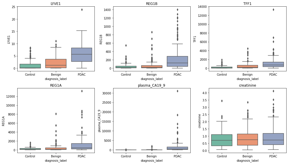

췌장암 환자 PDAC
- LYVE1이 높음. REG1B가 높음 TFF1이 높음, REF1A가 높음

Spearman Correlation

corr = df[biomarkers].corr(method="spearman", min_periods=20)
plt.figure(figsize=(8,7))
plt.imshow(corr, aspect="auto", interpolation="nearest")
plt.xticks(range(len(biomarkers)), biomarkers, rotation=45, ha="right")
plt.yticks(range(len(biomarkers)), biomarkers)
plt.title("Spearman correlation (biomarkers)")
plt.colorbar()
plt.tight_layout()
plt.show()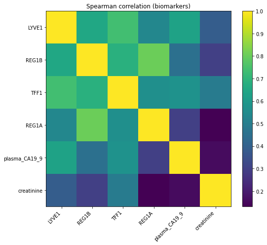

Statistical Test

for biomarker in biomarkers:
    groups = [df[df['diagnosis_label'] == g][biomarker].dropna() for g in df['diagnosis_label'].unique()]
    stat, p = f_oneway(*groups)
    print(f"{biomarker}: p-value = {p:.4f}")

LYVE1: p-value = 0.0000
REG1B: p-value = 0.0000
TFF1: p-value = 0.0000
REG1A: p-value = 0.0000
plasma_CA19_9: p-value = 0.0000
creatinine: p-value = 0.1894

dignose level 별로 그룹 간 차이가 있는지
- creatime 빼고 다 차이 있음

Random Forest

target, features

X = df[biomarkers].fillna(0)
y = df['diagnosis']

X_train, X_test, y_train, y_test = train_test_split(X, y, test_size=0.2, random_state=42)

randomforest

rf = RandomForestClassifier(random_state=42)
rf.fit(X_train, y_train)

RandomForestClassifier(random_state=42)

In a Jupyter environment, please rerun this cell to show the HTML representation or trust the notebook.
On GitHub, the HTML representation is unable to render, please try loading this page with nbviewer.org.

prediction

y_pred = rf.predict(X_test)
print(classification_report(y_test, y_pred))

              precision    recall  f1-score   support

           1       0.76      0.76      0.76        41
           2       0.61      0.59      0.60        39
           3       0.85      0.87      0.86        38

    accuracy                           0.74       118
   macro avg       0.74      0.74      0.74       118
weighted avg       0.74      0.74      0.74       118

Confusion Matrix

cm = confusion_matrix(y_test, y_pred, labels=[1,2,3])
plt.figure(figsize=(7,6))
plt.imshow(cm, interpolation="nearest")
plt.title("Confusion Matrix (RF)")
plt.xticks([0,1,2], ["1-Control","2-Benign","3-PDAC"], rotation=20)
plt.yticks([0,1,2], ["1-Control","2-Benign","3-PDAC"])
for i in range(3):
    for j in range(3):
        plt.text(j, i, cm[i, j], ha="center", va="center")
plt.colorbar()
plt.tight_layout()
plt.show()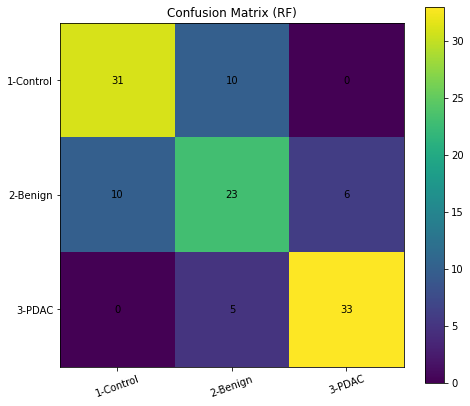

Check Feature Importance

importances = pd.Series(rf.feature_importances_, index=biomarkers).sort_values(ascending=False)
importances

plasma_CA19_9    0.241888
LYVE1            0.216604
TFF1             0.181022
REG1B            0.146198
creatinine       0.123882
REG1A            0.090405
dtype: float64

sns.barplot(x=importances, y=importances.index)
plt.title('Feature Importance')
plt.show()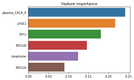

Logistic Regression

feature_cols = ["age", "creatinine", "LYVE1", "REG1B", "TFF1", "REG1A", "plasma_CA19_9"]
X = df[feature_cols].copy()
X["sex"] = df["sex"].map({"M":0, "F":1})
y = df["diagnosis"]

X = X.fillna(X.median())
X_train, X_test, y_train, y_test = train_test_split(
    X, y, test_size=0.25, random_state=42, stratify=y
)

log_reg = Pipeline([
    ('scaler', StandardScaler()),
    ('clf', LogisticRegression(max_iter=200, multi_class='ovr'))
])
log_reg.fit(X_train, y_train)
print("\n--- Logistic Regression ---")
print(classification_report(y_test, log_reg.predict(X_test)))


--- Logistic Regression ---
              precision    recall  f1-score   support

           1       0.62      0.63      0.62        46
           2       0.60      0.52      0.56        52
           3       0.75      0.84      0.79        50

    accuracy                           0.66       148
   macro avg       0.66      0.66      0.66       148
weighted avg       0.66      0.66      0.66       148

svm = Pipeline([
    ('scaler', StandardScaler()),
    ('clf', SVC(kernel='rbf', probability=True))
])
svm.fit(X_train, y_train)
print("\n--- SVM (RBF kernel) ---")
print(classification_report(y_test, svm.predict(X_test)))


--- SVM (RBF kernel) ---
              precision    recall  f1-score   support

           1       0.61      0.72      0.66        46
           2       0.64      0.48      0.55        52
           3       0.76      0.84      0.80        50

    accuracy                           0.68       148
   macro avg       0.67      0.68      0.67       148
weighted avg       0.67      0.68      0.67       148

for name, model in [("LR", log_reg), ("SVM", svm)]:
    y_proba = model.predict_proba(X_test)
    auc = roc_auc_score(pd.get_dummies(y_test), y_proba, multi_class='ovr')
    print(f"log_reg macro AUC: {auc:.3f}")

log_reg macro AUC: 0.849
log_reg macro AUC: 0.843

AUC 별 차이 없음

biomarkers = ["age", "creatinine", "LYVE1", "REG1B", "TFF1", "REG1A", "plasma_CA19_9"]
X = df[biomarkers].copy()
X["sex"] = df["sex"].map({"M":0, "F":1})
y = df["diagnosis"] - 1   # 0,1,2 로 바꿈 (PyTorch용)

X = X.fillna(X.median())
scaler = StandardScaler()
X_scaled = scaler.fit_transform(X)

X_train, X_test, y_train, y_test = train_test_split(X_scaled, y, test_size=0.25, random_state=42, stratify=y)

X_train = torch.tensor(X_train, dtype=torch.float32)
y_train = torch.tensor(y_train.values, dtype=torch.long)
X_test = torch.tensor(X_test, dtype=torch.float32)
y_test = torch.tensor(y_test.values, dtype=torch.long)

data loader

class BiomarkerDataset(Dataset):
    def __init__(self, X, y):
        self.X = X
        self.y = y
    def __len__(self):
        return len(self.X)
    def __getitem__(self, idx):
        return self.X[idx], self.y[idx]

train_dataset = BiomarkerDataset(X_train, y_train)
test_dataset = BiomarkerDataset(X_test, y_test)

train_loader = DataLoader(train_dataset, batch_size=16, shuffle=True)
test_loader = DataLoader(test_dataset, batch_size=16, shuffle=False)

class MLPClassifier(nn.Module):
    def __init__(self, input_dim, hidden_dims=[128, 64, 32], output_dim=3, dropout=0.4):
        super().__init__()
        self.layers = nn.Sequential(
            nn.Linear(input_dim, hidden_dims[0]),
            nn.ReLU(),
            nn.Dropout(dropout),
            nn.Linear(hidden_dims[0], hidden_dims[1]),
            nn.ReLU(),
            nn.Dropout(dropout),
            nn.Linear(hidden_dims[1], hidden_dims[2]),
            nn.ReLU(),
            nn.Dropout(dropout),
            nn.Linear(hidden_dims[2], output_dim)
        )
    def forward(self, x):
        return self.layers(x)

input_dim = X_train.shape[1]
model = MLPClassifier(input_dim=input_dim)
device = torch.device("cuda" if torch.cuda.is_available() else "cpu")
model = model.to(device)

criterion = nn.CrossEntropyLoss()
optimizer = optim.Adam(model.parameters(), lr=0.001)
epochs = 100

train_losses, test_losses = [], []

for epoch in range(epochs):
    model.train()
    total_loss = 0
    for X_batch, y_batch in train_loader:
        X_batch, y_batch = X_batch.to(device), y_batch.to(device)
        optimizer.zero_grad()
        output = model(X_batch)
        loss = criterion(output, y_batch)
        loss.backward()
        optimizer.step()
        total_loss += loss.item()
    train_losses.append(total_loss / len(train_loader))

    # Validation loss
    model.eval()
    val_loss = 0
    with torch.no_grad():
        for X_batch, y_batch in test_loader:
            X_batch, y_batch = X_batch.to(device), y_batch.to(device)
            output = model(X_batch)
            val_loss += criterion(output, y_batch).item()
    test_losses.append(val_loss / len(test_loader))

    if epoch % 10 == 0:
        print(f"Epoch [{epoch}/{epochs}] Train Loss: {train_losses[-1]:.4f}  Val Loss: {test_losses[-1]:.4f}")

Epoch [0/100] Train Loss: 1.0805  Val Loss: 1.0263
Epoch [10/100] Train Loss: 0.7961  Val Loss: 0.7018
Epoch [20/100] Train Loss: 0.7519  Val Loss: 0.6944
Epoch [30/100] Train Loss: 0.6993  Val Loss: 0.6584
Epoch [40/100] Train Loss: 0.7230  Val Loss: 0.6667
Epoch [50/100] Train Loss: 0.6858  Val Loss: 0.6535
Epoch [60/100] Train Loss: 0.6685  Val Loss: 0.6601
Epoch [70/100] Train Loss: 0.6517  Val Loss: 0.6542
Epoch [80/100] Train Loss: 0.6436  Val Loss: 0.6437
Epoch [90/100] Train Loss: 0.6599  Val Loss: 0.6618

plt.plot(train_losses, label="Train Loss")
plt.plot(test_losses, label="Val Loss")
plt.legend()
plt.title("Training Curve")
plt.xlabel("Epoch")
plt.ylabel("Loss")
plt.show()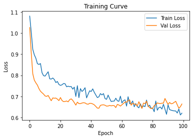

model.eval()

MLPClassifier(
  (layers): Sequential(
    (0): Linear(in_features=8, out_features=128, bias=True)
    (1): ReLU()
    (2): Dropout(p=0.4, inplace=False)
    (3): Linear(in_features=128, out_features=64, bias=True)
    (4): ReLU()
    (5): Dropout(p=0.4, inplace=False)
    (6): Linear(in_features=64, out_features=32, bias=True)
    (7): ReLU()
    (8): Dropout(p=0.4, inplace=False)
    (9): Linear(in_features=32, out_features=3, bias=True)
  )
)

with torch.no_grad():
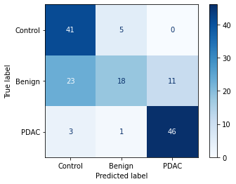
    preds = model(X_test.to(device)).argmax(dim=1).cpu().numpy()

print(classification_report(y_test, preds, target_names=["Control","Benign","PDAC"]))

              precision    recall  f1-score   support

     Control       0.61      0.89      0.73        46
      Benign       0.75      0.35      0.47        52
        PDAC       0.81      0.92      0.86        50

    accuracy                           0.71       148
   macro avg       0.72      0.72      0.69       148
weighted avg       0.73      0.71      0.68       148

cm = confusion_matrix(y_test, preds)
disp = ConfusionMatrixDisplay(cm, display_labels=["Control","Benign","PDAC"])
disp.plot(cmap="Blues")
plt.show()